Technology of Acoustic Scintillation Flow Meter

Technology

Measurement principles Features and benefits Measurement description Conditions of use

Measurement principles

Acoustic scintillation drift is a technique for measuring flow in a turbulent medium by analyzing the variations in ultrasonic pulses that have been transmitted through the medium.

The Acoustic Scintillation Flow Meter (ASFM) uses this technique to measure the velocity of the water flowing through a conduit (e.g. an intake to a hydroelectric turbine) by utilizing the turbulence in the flow (e.g. small-scale turbulence generated by the intake trash racks).

With two transmitters placed at one side of the conduit, and two receivers at the other, the signal amplitude at the receivers will vary randomly in time as the distribution of turbulence along the propagation paths changes with time and the flow. If the paths are sufficiently closely spaced, the turbulence will remain embedded in the flow, and the pattern of the variations (known as “scintillations”) at the downstream receiver will be nearly identical to that at the upstream receiver, except for a time delay, Δ_t (Fig 1). If these scintillations are examined over a suitable time period, this time delay can be determined. The mean flow velocity perpendicular to the acoustic path is then Δ_x/Δ_t, where Δ_x is the separation between the paths. Using three receivers in a triangular array allows both the magnitude and inclination of the laterally averaged velocity to be measured.

The average velocity is measured at several pre-selected measurement levels. Total flow rate is calculated by integrating the average horizontal component of the velocity at each level over the total cross-sectional area of the conduit.

Fundamentals of Acoustic Scintillation video (mpg) (wmv)

Figure 1: Simplified representation
of time delay measurement by
acoustic scintillation

Features and benefits of the technology

Does not require long straight sections of conduit	Well suited to low-head plants where intakes are short and rapidly converging or equipped with fish diversion structures but can be used at higher-head plants with suitable intakes as well.
Accurate and repeatable	Comparative measurements with other technologies (such as current meters or acoustic time of flight) confirm that in suitable applications, ASFM accuracy and precision are within code acceptable limits
Uses spatial averaging	Large scale eddies and meandering do not bias the measurements
Non-intrusive	No instruments are placed in the measurement zone, avoiding interference with the flow and impact by floating debris, thus suitable for long-term monitoring
No moving parts	Does not require mechanical maintenance or periodic calibration
Cost-effective	If stoplog or gate slots are available, can be installed on frames in the yard. No dewatering of the intake is required. Fully instrumented frames can be moved between identical intakes. Operational downtime and measurement cost are minimized (GMS study)
User friendly	Easy to operate. Velocity and discharge data displays are available immediately

Measurement description

In multi-bay intakes, the ASFM measures the flow velocity simultaneously at one measurement path in each measurement section. The acoustic transducers (transmitters and receivers) are placed so that the paths are at the same nominal elevation in each intake bay, and sampling occurs at one such measurement path simultaneously in each bay. After sampling at the first measurement path is complete, the ASFM computes the flow velocity for that path and then switches to the next measurement path. The process is repeated until all measurement paths in the measurement section have been sampled. The typical sequence is from the floor to the roof. When sampling and individual velocity calculations are completed, the discharge is computed for each bay. Discharges in individual bays are then added arithmetically to produce the total discharge for the operating condition being measured. The results (discharges and the flow velocities and inclinations) are written to an electronic file, and the ASFM is ready for a new measurement.

ASFM requires a minimum sample size to produce a statistically meaningful measurement. The sampling period should be of sufficient duration to average out turbulent fluctuations. At least three or four data collection cycles at each measurement path are recommended to permit calculation of an average discharge and standard deviation.

Figure. 2 ASFM Typical arrangement- fixed frame
(Click on image to enlarge)

There are two basic approaches to measurement paths placement: a number of measurement paths at fixed elevations on a fixed-frame spanning the full height of the measurement section (Fig 2), or one or more paths mounted on a smaller profiling frame that is moved through a series of elevations to sample the full height of the measurement section (Fig. 3).

In a fixed-frame installation, the individual measurement paths are placed to optimally sample the vertical structure of the flow. It is recommended that uniform 1.5 m spacing of the measurement paths be used, except in regions where large variations in velocity are expected, where closer spacing will be beneficial. The integration algorithm used for computations does not require regular spacing of the sampling paths.

moving frame

Figure. 3 ASFM Typical arrangement- profiling frame

Profiling frames may be either stopped at each measurement position for the duration of the measurement or, if using a very slow (not more than 25 mm/sec) and constant travel speed, swept continuously over the total vertical dimension of the measurement section. If a continuous sweep is used, the position of the frame as a function of time must be recorded electronically. In general, profiling frames allow more flexibility in measurement path locations, but at the inconvenience of having frame cross-members in the flow.

It is also possible to attach the transducers directly to the intake side walls, but that would normally only be done if a permanent installation is intended or no intake slots are available.

The measurement paths must not be placed too close to boundaries, such as the floor and roof, because of interfering echoes. The limit of approach depends on the width of the measurement section. To ensure proper sampling near these boundaries, the uppermost and lowermost measurement paths should be positioned at the distances D:

D = (Wcτ/2)^½

where W is the width of the measurement section, c is the speed of sound and τ is the duration of the acoustic pulse (16 μsec is a typical value for τ, and cτ may usually be approximated by 0.024). This limit also applies to the distance between the measurement paths and the mounting frame cross-members. Uncertainties can be reduced when the number of measurement paths is increased. As many as 30 paths can be used in one measurement section when the intake characteristics and the desired accuracy so dictate.

Conditions of use

A) General

The ASFM has been developed specifically for the short, rectangular converging intakes typically found in plants with heads of 35 meters or less. However, the ASFM may be used at higher head plants when the intake characteristics comply with the requirements of this section. Because of the unstable inflow velocities or divergent approach angles likely existing in most intake measurement locations, both the magnitude and the direction of the velocities measured by the ASFM must be considered in the calculation of discharge.
A critical assumption of the ASFM measurement technology is that the intensity and spectral characteristics of the turbulence in the moving fluid are uniformly distributed along the acoustic transmission paths. Such turbulence is usually present downstream of trash racks with fine vertical members. The following site-specific intake characteristics must be considered individually:

Variations in the size and shape of the trashrack structural supports upstream of the ASFM measurement plane, and their distance from the measurement plane.
Variations in the uniformity and directionality of the inflow.
Shape irregularities upstream and downstream of the measurement plane.

B) Intakes for which accurate results can be obtained directly
Experience has shown that the ASFM produces accurate and repeatable results when the following conditions are complied with:

Trash racks vertical structural supports are less than 100 mm in width or more than 6.0 m from the measurement plane and the trash racks have been cleaned prior to the testing.
The horizontal angle between the inflow velocity vector and the axis of the intake does not exceed 15 degrees, and the operation of the neighbouring units and the spillway, if applicable, is controlled to the degree necessary to remain within this limitation during the period required to perform the measurements.
Average flow velocities are between 0.5 and 8.5 m/s and measurement sections are wider than 1.5 m.
There are no non-typical intake conduit shapes, particularly those that can result in recirculation. The presence of such irregularities must be investigated before starting the measurement.
Fish diversion screens upstream of the measurement plane will require special investigations.
There are no excessive air bubbles and/or acoustic noise. If their presence results in missed samples, enough valid samples must be obtained to be compatible with the assumptions used in the error analysis.

C) Intakes for which bias corrections will be required
For some intakes where the above requirements are not fulfilled, the systematic uncertainty of the measurement may be predicted before the measurement is started, and thus removed from the measurement results, as follows:

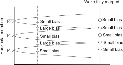
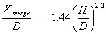
In a normal ASFM installation, the measurement paths are horizontal, and thus large vertical trash rack supports can introduce bias into the ASFM measurements. As illustrated in Fig. 4, the magnitude of the measurement bias is strongly dependent on the contrast between the turbulence of the intersecting vertical wakes and the turbulence within the remainder of the acoustic path, the distance between the measurement plane and the trash rack support and the width of the trash rack supports. If the wakes from the major horizontal trash rack supports (parallel to the acoustic paths) have merged before they reach the measurement plane, then it is very likely that the bias due to the wakes from the vertical support members will be reduced to a negligible amount. The distance downstream of the trash rack, X_merge required for the wakes from the horizontal members to merge may be estimated as

where
H is the vertical separation between the major horizontal trash rack supports,
D is their width in the vertical and
X is the distance between the trash rack and the measurement plane (all dimensions in meters).

If the distance to the measurement section is less than X_merge, an upper bound for the bias error due to wakes from the vertical members may be estimated using numerical calculations (Bouhadji et al. 2003) and comparisons with the available experimental data on similar structures (Wygnanski, I. J., Champagne, F., and Marasli, B. 1986. On the Large Scale Structures in Two-Dimensional, Small-Deficity, Turbulent Wakes. J.Fluid Mech. 168, 31-71 and Stewart, R. W., and A. A. Townsend, 1951. Similarity and self preservation in isotropic turbulence. Phil. Trans. Roy. Soc. London, A243, 359-386.)

Figure. 4: Illustration of the relation between wake merging and ASFM bias

Experience has shown that with these corrections the resulting systematic uncertainty of measurements with the ASFM can be within
±2% for many difficult intakes which do not comply with the requirements of paragraph B above. However, experience has also shown that there will be some exceptionally difficult intakes where no acceptable measurement uncertainties will be achievable.

Field Comparison Measurements

In order to verify the accuracy of the ASFM, a number of comparison measurements were carried out. Their results are shown graphically below, and further details of the individual measurements can be found under appropriate headings in the Technical Reports section (http://aqflow.com/reports.html).

field comparison

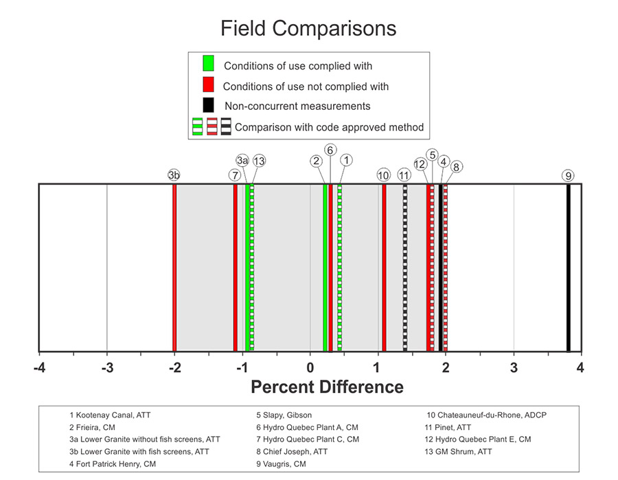
It can be noted that when the conditions of use listed in previous paragraphs are complied with, all four ASFM results agree with the reference measurements within ±1%. Even when the conditions of use are not complied with, all ASFM results agree with the reference measurements within ±2.0% (±2.0% indicated by shaded area). The only measurement outside the ±2.0% limits was a non-concurrent measurement at Vaugris, France.

More comparative measurements are needed; several are already in the planning stages. Nevertheless, the results to-date prove that the accuracy of the ASFM is comparable to other established and code-accepted measurement methods. Consequently, they are currently being reviewed in detail by the IEC 60041 and ASME PTC-18 code committees as part of their respective processes of publication updating. The IEC code is scheduled for re-publication in 2018, the ASME code is scheduled for re-publication in 2018. The acoustic scintillation measurement method will be included in both of these codes.